Matrix Comparisons¶

Ecopy contains several methods for comparing matrices. Some of these are similar to ordination, while others are more traditional null hypothesis testing.

Mantel (Mantel test)

anosim (Analysis of similarity)

simper() (Percentage similarity calculations)

procrustes_test (Procrustes test of matrix correlations)

corner4 (Fourth corner analysis)

rlq (RLQ analysis)

rda (RDA analysis)

cca (CCA analysis)

ccor (CCor analysis)

class Mantel(d1, d2, test='pearson', tail='both', nperm=999)¶

Takes two distance matrices for a Mantel test. Returns object of class Mantel. Calculates the cross-product between lower triangle matrices, using either standardized variables or standardized ranks. The test statistics is the cross-product is divided by

$\frac{n(n-1)}{2} - 1$

where n is the number of objects.

Parameters

d1: numpy.ndarray or pandas.DataFrame

First distance matrix.

d2: numpy.nadarray or pandas.DataFrame

Second distance matrix.

test: [‘pearson’ | ‘spearman’]

‘pearson’ performs Mantel test on standardized variables.

‘spearman’ performs Mantel test on standardized ranks.

tail: [‘both’ | ‘greater’ | ‘lower’]

‘greater’ tests the one-tailed hypothesis that correlation is greater than predicted.

‘lower’ tests hypothsis that correlation is lower than predicted.

‘both’ is a two-tailed test.

nperm: int

Number of permutations for the test.

Attributes

r_obs¶: Observed correlation statistic.

pval¶: p-value for the given hypothesis.

tail¶: The tested hypothesis.

test¶: Which of the statistics used, ‘pearson’ or ‘spearman’.

perm¶: Number of permutations.

Methods

classmethod summary()¶: Prints a summary output table.

Examples

Load the data:

import ecopy as ep
v1 = ep.load_data('varespec')
v2 = ep.load_data('varechem')

Standardize the chemistry variables and calculate distance matrices:

v2 = v2.apply(lambda x: (x - x.mean())/x.std(), axis=0)
dist1 = ep.distance(v1, 'bray')
dist2 = ep.distance(v2, 'euclidean')

Conduct the Mantel test:

mant = ep.Mantel(dist1, dist2)
print mant.summary()

Pearson Mantel Test
Hypothesis = both

Observed r = 0.305      p = 0.004
999 permutations

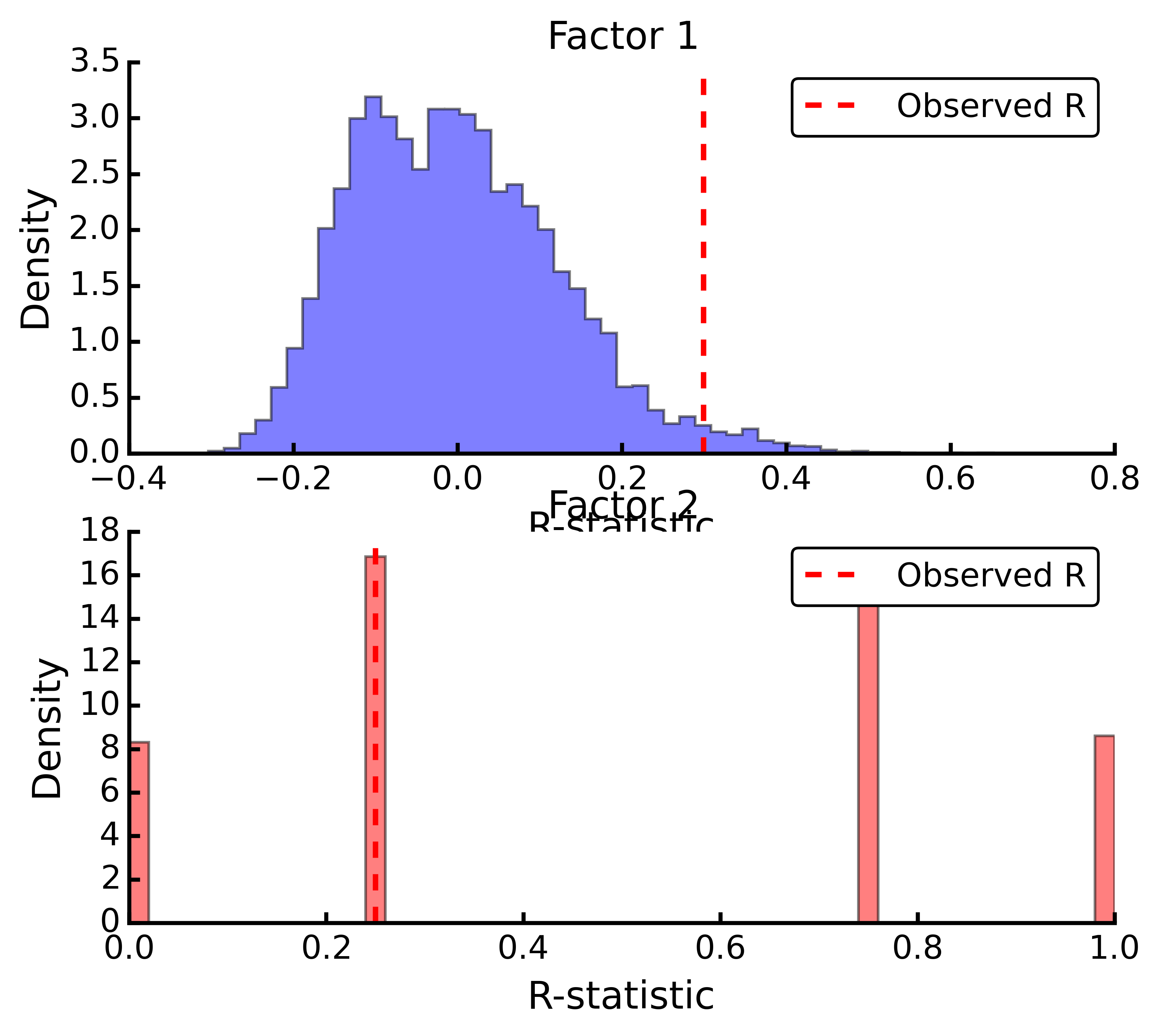
class anosim(dist, factor1, factor2=None, nested=False, nperm=999)¶

Conducts analysis of similarity (ANOSIM) on a distance matrix given one or two factors (groups). Returns object of anosim. Calculates the observed R-statistic as

$R = \frac{r_b - r_w}{\frac{n(n-1)}{4}}$

where $r_w$ is the average within-group ranked distances, $r_b$ is the average between-group ranked distances, and n is the number of objects (rows) in the distance matrix. The factor is then randomly permuted and R recalculated to generate a null distribution.

Parameters

dist: numpy.ndarray or pandas.DataFrame: Square-symmetric distance matrix.
factor1: numpy.nadarray or pandas.Series or pandas.DataFrame: First factor.
factor2: numpy.nadarray or pandas.Series or pandas.DataFrame: Second factor.
nested: [True | False]: Whether factor1 is nested within factor2. If False, then factor1 and factor2 are permuted independently. If Tue, then factor1 is permuted only within groupings of factor2.
nperm: int: Number of permutations for the test.

Attributes

r_perm1¶: Permuted R-statistics for factor1.

r_perm2¶: Permuted R-statistics for factor1.

R_obs1¶: Observed R-statistic for factor1.

R_obs2¶: Observed R-statistic for factor2.

pval¶: List of p-values for factor1 and factor2.

perm¶: Number of permutations.

Methods

classmethod summary()¶: Prints a summary output table.

classmethod plot()¶: Plots a histogram of R values.

Examples

Load the data:

import ecopy as ep
data1 = ep.load_data('dune')
data2 = com.load_data('dune_env')

Calculate Bray-Curtis dissimilarity on the ‘dune’ data, save the ‘Management’ factor as factor1 and generate factor2:

duneDist = ep.distance(data1, 'bray')
group1 = data2['Management']
group2map = {'SF': 'A', 'BF': 'A', 'HF': 'B', 'NM': 'B'}
group2 = group1.map(group2map)

Conduct the ANOSIM:

t1 = ep.anosim(duneDist, group1, group2, nested=True, nperm=9999)
print t1.summary()

ANOSIM: Factor 1
Observed R = 0.299
p-value = 0.0217
9999 permutations

ANOSIM: Factor 2
Observed R = 0.25
p-value = 0.497
9999 permutations

t1.plot()

simper(data, factor, spNames=None)¶

Conducts a SIMPER (percentage similarity) analysis for a site x species matrix given a grouping factor. Returns a pandas.DataFrame containing all output for each group comparison. Percent similarity for each species is calculated as the mean Bray-Curtis dissimilarity of each species, given by:

$\Delta_i = \frac{|y_{ik} - y_{ij}|}{\sum_i^n (y_{ik} + y_{ij})}$

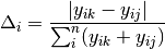
The denominator is the total number of individuals in both sites, $y_{ik}$ is the number of individuals of species i in site k, and $y_{ij}$ is the number of individuals in site j. This is performed for every pairwise combination of sites across two groups and then averaged to yield the mean percentage similarity of the species. This function also calculates the standard deviation of the percentage similarity, the signal to noise ratio (mean / sd) such that a higher ratio indicates more consistent difference, the percentage contribution of each species to the overall difference, and the cumulative percentage difference.

The output is a multi-indexed DataFrame, with the first index providing the comparison and the second index providing the species. The function lists the index comparison names as it progresses for reference.

Parameters

data: numpy.ndarray or pandas.DataFrame: A site x species matrix.
factor: numpy.nadarray or pandas.Series or pandas.DataFrame or list: Grouping factor.
spNames: list: List of species names. If data is a pandas.DataFrame, then spNames is inferred as the column names. If data is a np.ndarray, then spNames is given integer values unless this argument is provided.

Examples

Conduct SIMPER on the ANOSIM data from above:

import ecopy as ep

data1 = ep.load_data('dune')
data2 = com.load_data('dune_env')
group1 = data2['Management']
fd = ep.simper(np.array(data1), group1, spNames=data1.columns)

Comparison indices:
BF-HF
BF-NM
BF-SF
HF-NM
HF-SF
NM-SF

print fd.ix['BF-NM']

 sp_mean  sp_sd  ratio  sp_pct  cumulative
Lolipere     9.07   2.64   3.44   12.43       12.43
Poatriv      5.47   4.46   1.23    7.50       19.93
Poaprat      5.25   1.81   2.90    7.19       27.12
Trifrepe     5.13   2.76   1.86    7.03       34.15
Bromhord     3.97   2.92   1.36    5.44       39.59
Bracruta     3.57   2.87   1.24    4.89       44.48
Eleopalu     3.38   3.57   0.95    4.63       49.11
Agrostol     3.34   3.47   0.96    4.58       53.69
Achimill     3.32   2.34   1.42    4.55       58.24
Scorautu     3.14   2.03   1.55    4.30       62.54
Anthodor     2.81   3.29   0.85    3.85       66.39
Planlanc     2.73   2.19   1.25    3.74       70.13
Salirepe     2.68   2.93   0.91    3.67       73.80
Bellpere     2.35   1.91   1.23    3.22       77.02
Hyporadi     2.17   2.45   0.89    2.97       79.99
Ranuflam     2.03   2.28   0.89    2.78       82.77
Elymrepe     2.00   2.93   0.68    2.74       85.51
Callcusp     1.78   2.68   0.66    2.44       87.95
Juncarti     1.77   2.60   0.68    2.43       90.38
Vicilath     1.58   1.45   1.09    2.17       92.55
Sagiproc     1.54   1.86   0.83    2.11       94.66
Airaprae     1.34   1.97   0.68    1.84       96.50
Comapalu     1.07   1.57   0.68    1.47       97.97
Alopgeni     1.00   1.46   0.68    1.37       99.34
Empenigr     0.48   1.11   0.43    0.66      100.00
Rumeacet     0.00   0.00    NaN    0.00      100.00
Cirsarve     0.00   0.00    NaN    0.00      100.00
Chenalbu     0.00   0.00    NaN    0.00      100.00
Trifprat     0.00   0.00    NaN    0.00      100.00
Juncbufo     0.00   0.00    NaN    0.00      100.00

class procrustes_test(mat1, mat2, nperm=999)¶

Conducts a procrustes test of matrix associations on two raw object x descriptor matrices. Returns an object of class procrustes_test. First, both matrices are column-centered. Then, each matrix is divided by the square root of its sum-of-squares. The test statistic $m_{12}^2$ is calculated as:

$m_{12}^2 = 1 - (Trace \mathbf{W})^2$

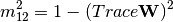
$\mathbf{W}$ is the diagonal matrix of eigenvalues for $\mathbf{X'Y}$ , which are the two transformed matrices. Then, rows of X are randomly permuted and the test statistic recalculated. The p-value is the the proportion of random test statistics less than the observed statistic.

Parameters

mat1: numpy.ndarray or pandas.DataFrame: A raw object x descriptor (site x species) matrix.
factor1: numpy.nadarray or pandas.DataFrame: A raw object x descriptor (site x descriptor) matrix.
nperm: int: Number of permutations in the test.

Attributes

m12_obs¶: Observed $m_{12}^2$ statistic.

pval¶: p-value.

perm¶: Number of permutations.

Methods

classmethod summary()¶: Prints a summary output table.

Examples

Load the data and run the Mantel test:

import ecopy as ep

d1 = ep.load_data('varespec')
d2 = ep.load_data('varechem')
d = ep.procrustes_test(d1, d2)
print d.summary()

m12 squared = 0.744
p = 0.00701

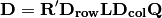
class corner4(mat1, mat2, nperm=999, model=1, test='both', p_adjustment=None)¶

Conducts fourth corner analysis examining associations between species traits and environmental variables. Species traits are given in a species x trait matrix Q, species abundances given in a site x species matrix L, and environmental traits given in a site x environment matrix R. The general concept of fourth corner analysis is to find matrix D:

$\begin{bmatrix} \mathbf{L} & \mathbf{R} \\ \mathbf{Q'} & \mathbf{D} \end{bmatrix}$

In a simple case, R and Q contain one environmental variable and one species trait. An expanded correspondance matrix is created following Dray and Legendre (2008). The association between R and Q is the calculated as follows:

If both variables are quantitative, then association is described by Pearson’s correlation coefficient r
If both variables are qualitative, then association is described by $\chi^2$ from a contingency table (see Dray and Legendre 2008, Legendre and Legendre 2011)
If one variable is quantitative but the other is qualitative, then association is described using the F-statistic.

Significance of the statistics is determined using one of four permutation models (see below).

If R and Q contain more than one variable or trait, then the test iterates through all possible environment-trait combinations. The method automatically determines the appropriates statistics, depending on the data types (float=quantitative or object=qualitative). NOTE: As of now, this is quite slow if the number of traits and/or environmental variables is large.

Parameters

R: pandas.DataFrame

A site x variable matrix containing environmental variables for each site. pandas.Series NOT allowed.

L: numpy.nadarray or pandas.DataFrame

A site x species matrix of either presence/absence or abundance. Only integer values allowed.

Q: pandas.DataFrame

A species x trait matrix containing trait measurements for each species. pandas.Series NOT allowed.

nperm: int

Number of permutations in the test.

model: [1 | 2 | 3 | 4]

Which model should be used for permutations.

1: Permutes within columns of L only (that is, shuffles species among sites).

2: Permutes entire rows of L (that is, shuffles entire species assemblages).

3: Permutes within rows of L (that is, shuffles the distribution of individuals within a site).

4: Permutes entire columns of L (that is, shuffles a species’ distribution among traits, while site distributions are kept constant).

test: [‘both’ | ‘greater’ | ‘lower’]

Which tail of the permutation distribution should be tested against the observed statistic.

p_adjustment: [None, ‘bonferroni’, ‘holm’, ‘fdr’]:

Which adjustment should be used for multiple comparisons. ‘bonferroni’ uses Bonferronni correction, ‘holm’ uses the Bonferroni-Holm correction, and ‘fdr’ uses the False Discovery Rate correction.

Methods

classmethod summary()¶: Returns a pandas.DataFrame of output.

Examples

Run fourth corner analysis on the aviurba data from R’s ade4 package:

import ecopy as ep

traits = ep.load_data('avi_traits')
env = ep.load_data('avi_env')
sp = ep.load_data('avi_sp')

fourcorn = ep.corner4(env, sp, traits, nperm=99, p_adjustment='fdr')
results = fourcorn.summary()

print results[['Comparison','adjusted p-value']]
                Comparison  adjusted p-value
0         farms - feed.hab             1.000
1       farms - feed.strat             1.000
2         farms - breeding             1.000
3        farms - migratory             1.000
4     small.bui - feed.hab             0.322
5   small.bui - feed.strat             0.580
6     small.bui - breeding             1.000
7    small.bui - migratory             0.909
8      high.bui - feed.hab             0.111
...     .......                    ....
41  veg.cover - feed.strat             1.000
42    veg.cover - breeding             0.033
43   veg.cover - migratory             1.000

class rlq(R, L, Q, ndim=2)¶

Conducts RLQ analysis which examines associations between matrices R (site x environment) and Q (species x traits) as mediated by matrix L (site by species). In general, a matrix D is constructed by:

$\mathbf{D} = \mathbf{R'}\mathbf{D_{row}}\mathbf{L}\mathbf{D_{col}}\mathbf{Q}$

where $\mathbf{D_{row}}$ and $\mathbf{D_{col}}$ are diagonal matrices of row and column weights derived from matrix L. L is first transformed by dividing the matrix by the total number of individuals in the matrix. Column and row weights are given by the sum of columns and rows of the transformed matrix. Matrix L is then transformed by diving each column by the corresponding column weight, dividing each row by the corresponding row weight, and subtracting 1 from all elements. This transformed L matrix is used in the above equation to generate matrix D.

NOTE: Both R and Q can contain a mix of factor and quantitative variables. A dummy dataframe is constructed for both R and Q as in the Hill and Smith ordination procedure.

Matrix D is then subject to eigen decomposition, giving site (environment) and species (trait) scores, as well as loading vectors for both environmental and trait variables.

Parameters

R: pandas.DataFrame: A site x environment matrix for ordination, where objects are rows and descriptors/variables as columns. Can have mixed data types (both quantitative and qualitative). In order to account for factors, this method creates dummy variables for each factor and then assigns weights to each dummy column based on the number of observations in each column.
L: pandas.DataFrame: A site x species for ordination, where objects are rows and descriptors/variables as columns.
Q: pandas.DataFrame: A species x trait matrix for ordination, where objects are rows and descriptors/variables as columns. Can have mixed data types (both quantitative and qualitative). In order to account for factors, this method creates dummy variables for each factor and then assigns weights to each dummy column based on the number of observations in each column.
ndim: int: Number of axes and components to save.

Attributes

traitVecs¶: A pandas.DataFrame of trait loadings.

envVecs¶: A pandas.DataFrame of environmental loadings.

normedTraits¶: Species coordinates along each axis.

normedEnv¶: Site coordinates along each axis.

evals¶: Eigenvalues for all axes (not just saved ones).

Methods

classmethod summary()¶: Returns a data frame containing information about the principle axes.

classmethod biplot(xax=1, yax=2)¶

Create a biplot. The plot contains four subplots, one each for species scores, site scores, trait vectors, and environment vectors. Species scores are plotted from normedTraits, site scores are plotted from normedEnv, trait vectors are plotted from traitVecs, and environmental vectors are plotted from envVecs. Users can mix and match which vectors to overlay with which points manually using these four attributes.

xax: integer: Specifies which PC axis to plot on the x-axis,
yax: integer: Specifies which PC axis to plot on the y-axis.

Examples

RLQ analysis of the aviurba data:

vi_sp = ep.load_data('avi_sp')
avi_env = ep.load_data('avi_env')
avi_traits = ep.load_data('avi_traits')

rlq_test = ep.rlq(avi_env, avi_sp, avi_traits, ndim=2)
print rlq_test.summary().iloc[:,:3]

                    Axis 1    Axis 2    Axis 3
Std. Dev  0.691580  0.376631  0.272509
Prop Var  0.657131  0.194894  0.102031
Cum Var   0.657131  0.852026  0.954056

rlq_test.biplot()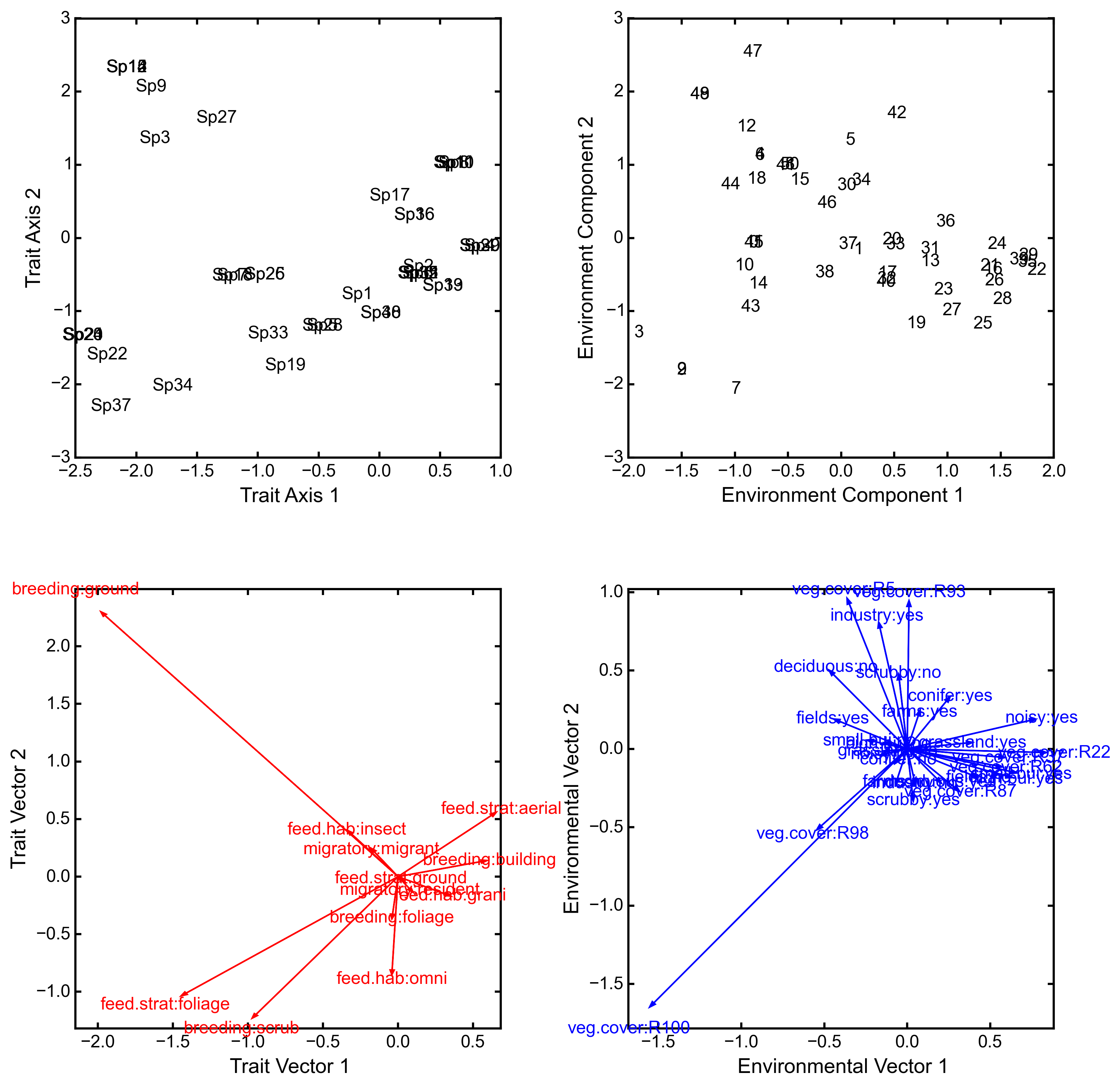

class rda(Y, X, scale_y=True, scale_x=False, design_x=False, varNames_y=None, varNames_x=None, rowNames=None, pTypes=None)¶

Conducts RDA analysis which examines the relationship between sites (rows) based on their species compositions (columns). This information is contained in matrix Y. However, the relationships between sites are constrained by environmental predictors contained in matrix X.

RDA performs a multivariate regression of Y against X, yielding linear predictors B:

$\mathbf{B} = (\mathbf{X}'\mathbf{X})^{-1}\mathbf{X}'\mathbf{Y}$

These linear predictors are used to generated predicted values for each species at each site:

$\mathbf{\hat{Y}} = \mathbf{XB}$

The variance-covariance matrix of $\mathbf{\hat{Y}}$ is then subject to eigen-analysis, yielding eigenvalues L and eigenvectors U of the predicted species values. Three new matrices are calculated:

$\mathbf{F} = \mathbf{YU} \mathbf{Z} = \mathbf{\hat{Y}U} \mathbf{C} = \mathbf{BU}$

Species scores are given by $\mathbf{U}\mathbf{L}^{-0.5}$ . Site scores are given by $\mathbf{F}\mathbf{L}^{-0.5}$ . The scores of each predictor are given in matrix C.

The residuals from the regression are then subject to PCA to ordinate the remaining, unconstrained variance.

Parameters

Y: pandas.DataFrame or numpy.ndarray: A site x species for ordination, where objects are rows and descriptors/variables as columns.
X: pandas.DataFrame or numpy.ndarray: A site x environment matrix for ordination, where objects are rows and descriptors/variables as columns. Only the pandas.DataFrame can have mixed data types (both quantitative and qualitative). In order to account for factors, this method creates dummy variables for each factor and then assigns weights to each dummy column based on the number of observations in each column.
scale_x: [True | False]: Whether or not the matrix Y should be standardized by columns.
scale_y: [True | False]: Whether or not the matrix X should be standardized by columns.
design_x: [True | False]: Whether or not X has already been transformed to a design matrix. This enables the user to formulate more complicated regressions that include interactions or higher order variables.
varNames_y: list: A list of variables names for each column of Y. If None, then the column names of Y are used.
varNames_x: list: A list of variables names for each column of X. If None, then the column names of X are used.
rowNames: list: A list of site names for each row. If none, then the index values of Y are used.
pTypes: list: A list denoting whether variables in X are quantitative (‘q’) or factors (‘f’). Can usually be ignored.

Attributes

spScores¶: A pandas.DataFrame of species scores on each RDA axis.

linSites¶: A pandas.DataFrame of linearly constrained site scores.

siteScores¶: A pandas.DataFrame of site scores on each RDA axis.

predScores¶: A pandas.DataFrame of predictor scores on each RDA axis.

RDA_evals¶: Eigenvalues for each RDA axis.

corr¶: Correlation of each predictor with each RDA axis.

resid_evals¶: Eigenvalues for residual variance.

resid_spScores¶: A pandas.DataFrame of species scores on PCA of residual variance.

resid_siteScores¶: A pandas.DataFrame of site scores on PCA of residual variance.

imp¶: Summary of importance of each RDA and PCA axis.

Methods

classmethod summary()¶: Returns a data frame containing summary information.

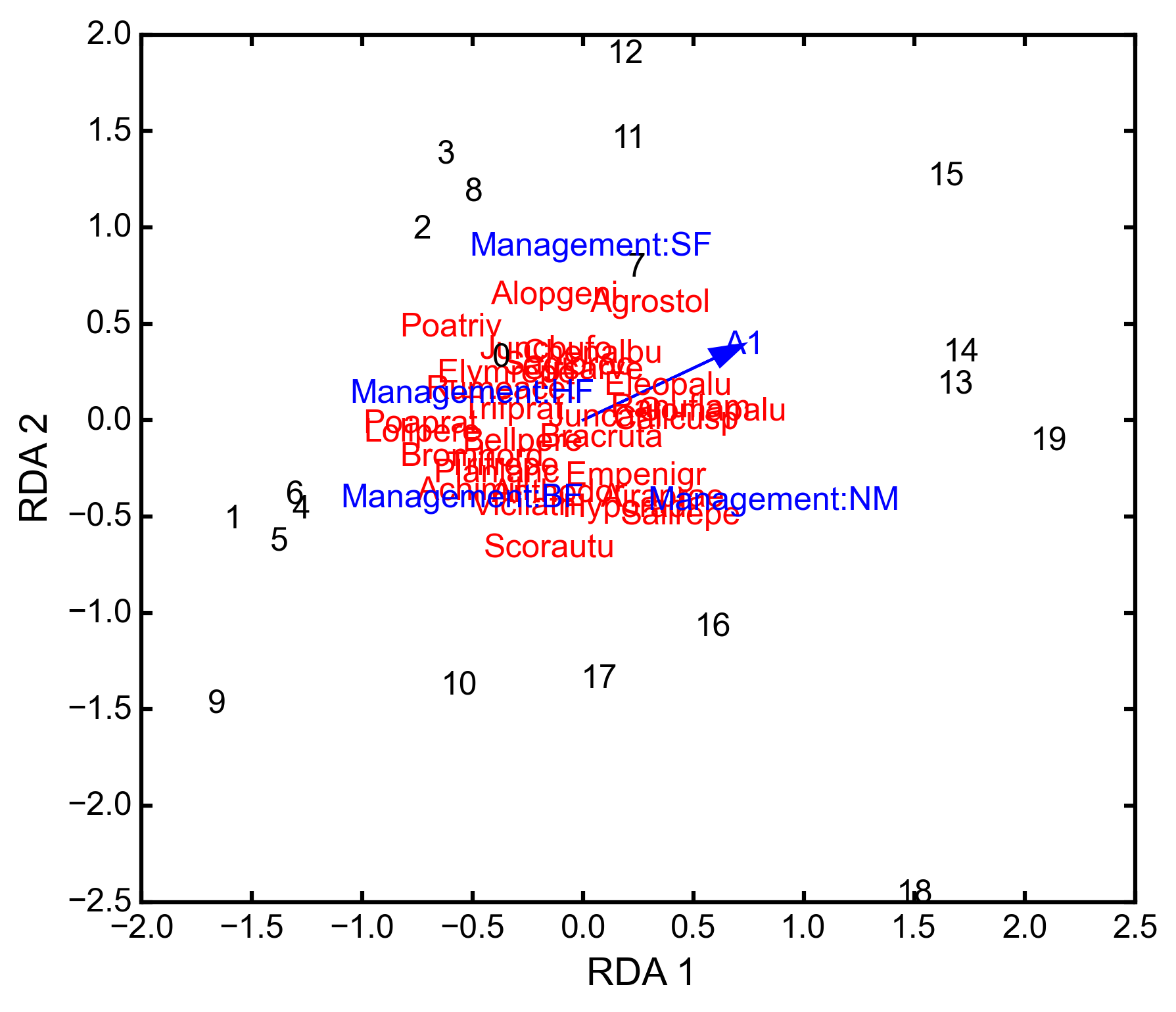
classmethod triplot(xax=1, yax=2)¶

Creates a triplot of species scores, site scores, and predictor variable loadings. If predictors are factors, they are represented by points. Quantitative predictors are represented by arrows.

xax: integer: Specifies which RDA axis to plot on the x-axis.
yax: integer: Specifies which RDA axis to plot on the y-axis.

Examples

RDA on dune data:

import ecopy as ep

dune = ep.load_data('dune')
dune_env = ep.load_data('dune_env')

RDA = ep.rda(dune, dune_env[['A1', 'Management']])
RDA.triplot()

class cca(Y, X, varNames_y=None, varNames_x=None, rowNames=None, scaling=1)¶

Conducts CCA analysis which examines the relationship between sites (rows) based on their species compositions (columns). This information is contained in matrix Y. However, the relationships between sites are constrained by environmental predictors contained in matrix X.

CCA first transforms the species matrix Y into matrix $\bar{\mathbf{Q}}$ as in correspondance analysis. The predictor matrix X is then standardized using the row weights from matrix Y to calculate the mean and standard deviation of each column, resulting in a new matrix $\mathbf{X}_{scale}$ . This matrix, along with a diagonal matrix of row weghts D is used in a multivariate regression of $\bar{\mathbf{Q}}$ against $\mathbf{X}_{scale}$ , yielding linear predictors B:

$\mathbf{B} = (\mathbf{X}_{scale}'\mathbf{DX}_{scale})^{-1}\mathbf{X}_{scale}'\mathbf{D^{0.5}Y}$

These linear predictors are used to generated predicted values for each species at each site:

$\mathbf{\hat{Y}} = \mathbf{D^{0.5}X_{scale}B}$

The cross-product matrix of $\mathbf{\hat{Y}}$ is then subject to eigen-analysis, yielding eigenvalues L and eigenvectors U of the predicted species values. Five new matrices are calculated using diagonal matrices of row $\mathbf{D}_{r}$ and column $\mathbf{D}_{c}$ weights:

$\hat{\mathbf{U}} = \bar{\mathbf{Q}}\mathbf{UL^{-0.5}} \mathbf{V} = \mathbf{D_c^{-0.5}U} \hat{\mathbf{V}} = \mathbf{D_r^{-0.5}}\hat{\mathbf{U}} \mathbf{F} = \hat{\mathbf{V}}\mathbf{L^{0.5}} \hat{\mathbf{F}} = \mathbf{VL^{0.5}}$

In scaling type 1, species scores are given by V and site scores are given by F. Fitted site scores are given by $\mathbf{D_r}\hat{\mathbf{Y}}\mathbf{U}$ . To calculate the predictor scores, the fitted site scores are standardized using row weights as was done for $\mathbf{X}_{scale}$ , yielding $\mathbf{Z}_{scale}$ . Predictor variable scores are then calculated as $\mathbf{X}_{scale}'\mathbf{D_rZ}_{scale}\mathbf{L^{0.5}}$ .

In scaling type 2, species scores are given by $\hat{\mathbf{F}}$ and site scores are given by $\hat{\mathbf{V}}$ . Fitted site scores are given by $\mathbf{D_r}\hat{\mathbf{Y}}\mathbf{UL^{-0.5}}$ . To calculate the predictor scores, the fitted site scores are standardized using row weights as was done for $\mathbf{X}_{scale}$ , yielding $\mathbf{Z}_{scale}$ . Predictor variable scores are then calculated as $\mathbf{X}_{scale}'\mathbf{D_rZ}_{scale}$ .

Residuals from the constrained ordination are available in order to subject them to CA.

Parameters

Y: pandas.DataFrame or numpy.ndarray: A pandas.DataFrame or numpy.ndarray containing species abundance data (site x species).
X: pandas.DataFrame or numpy.ndarray: A pandas.DataFrame or numpy.ndarray containing predictor variables for constrained ordination (site x variable).
varNames_y: list: A list of variables names for each column of Y. If None, then the column names of Y are used.
varNames_x: list: A list of variables names for each column of X. If None, then the column names of X are used.
rowNames: list: A list of site names for each row. If none, then the index values of Y are used.
scaling: [1 | 2]: Which scaling should be used. See above.

Attributes

r_w¶: Row weights.

c_w¶: Column weights.

evals¶: Constrained eigenvalues.

U¶: Constrained eigenvectors.

resid¶: A pandas.DataFrame of residuals from the constrained ordination.

spScores¶: A pandas.DataFrame of species scores.

siteScores¶: A pandas.DataFrame of site scores.

siteFitted¶: A pandas.DataFrame of constrained site scores.

varScores¶: A pandas.DataFrame variable scores.

Methods

classmethod summary()¶: Returns summary information of each CA axis.

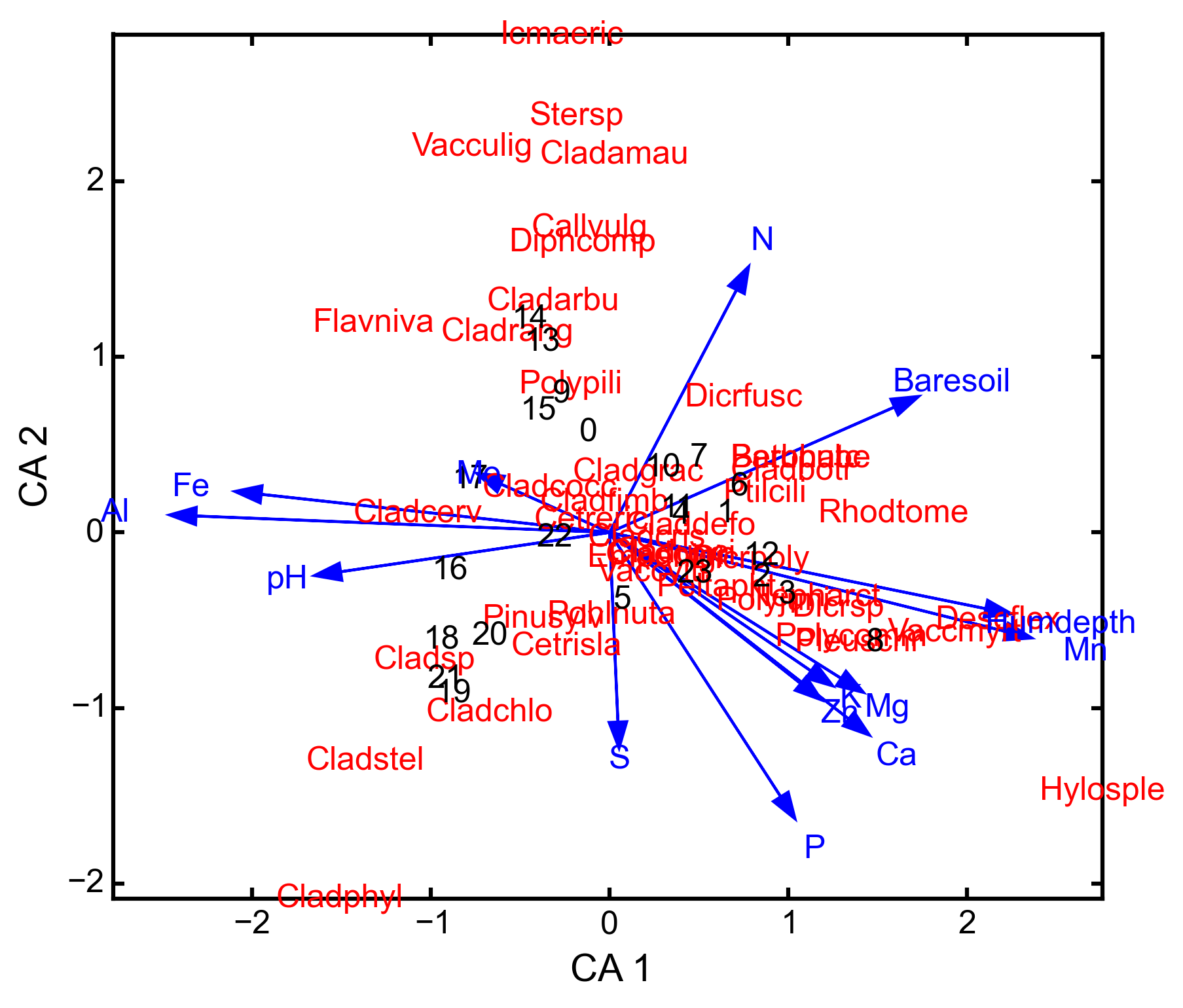
classmethod triplot(xax=1, yax=2)¶

Creates a triplot of species scores, site scores, and predictor variable loadings.

xax: integer: Specifies which CA axis to plot on the x-axis.
yax: integer: Specifies which Ca axis to plot on the y-axis.

Examples

CCA on varespec data:

import ecopy as ep

varespec = ep.load_data('varespec')
varechem = ep.load_data('varechem')

cca_fit = ep.cca(varespec, varechem)
CCA.triplot()

class ccor(self, Y1, Y2, varNames_1=None, varNames_2=None, stand_1=False, stand_2=False, siteNames=None)¶

Conducts canonical correlation analysis (CCor) which examines the relationship between matrices Y1 and Y2. CCor first calculates the variance and covariance matrices for both Y1 and Y2, where $\mathbf{S}_{11}$ is the variance-covariance matrix of Y1, $\mathbf{S}_{22}$ is the variance-covariance matrix of Y2, and $\mathbf{S}_{12}$ is the covariance matrix of Y1 and Y2.

A new matrix K is calculated as

$\mathbf{K} = \mathbf{S}_{11}^c \mathbf{S}_{12} \mathbf{S}_{22}^c$

where $\mathbf{S}_{11}^c$ is the Cholesky decomposition of $\mathbf{S}_{11}$ and same for $\mathbf{S}_{22}^c$ .

CCor then uses SVD to calculate matrices V, W, and U, where V contains the left-hand eigenvectors, W contains the singular values, and U contains the right-hand eigenvectors. New matrices C1 and C2 are derived by Y1V and Y2U, respectively. Scores for matrices Y1 are then

$\mathbf{\text{Scores}_1} = \mathbf{Y1C1}$

and the same for Y2. Variable loadings are the correlation between the original matrix and the scores.

Parameters

Y1: pandas.DataFrame or numpy.ndarray

A pandas.DataFrame or numpy.ndarray containing one set of variables.

Y2: pandas.DataFrame or numpy.ndarray

A pandas.DataFrame or numpy.ndarray containing a second set of variables.

varNames_1: list

A list of variables names for each column of Y1. If None, then the column names of Y1 are used.

varNames_2: list

A list of variables names for each column of Y2. If None, then the column names of Y2 are used.

siteNames: list

A list of site names for each row. If none, then the index values of Y1 are used.

stand_1: [True | False]

Whether to standardize Y1.

stand_2: [True | False]

Whether to standardize Y2.

Attributes

Scores1¶: Site scores from matrix 1.

Scores2¶: Site scores from matrix 2.

loadings1¶: Variable loadings from matrix 1.

loadings2¶: Variable loadings from matrix 2.

evals¶: Eigenvalues.

Methods

classmethod summary()¶: Returns summary information of each CA axis.

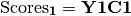
classmethod biplot(matrix=1, xax=1, yax=2)¶

Creates a biplot of site scores and predictor variable loadings.

matrix: [1 | 2]: Which matrix, Y1 or Y2 to plot.
xax: integer: Specifies which CCor axis to plot on the x-axis.
yax: integer: Specifies which CCor axis to plot on the y-axis.

Examples

CCor analysis of random data:

import ecopy as ep
import numpy as np

Y1 = np.random.normal(size=20*5).reshape(20, 5)
Y2 = np.random.normal(size=20*3).reshape(20, 3)

cc = ep.ccor(Y1, Y2)
cc.summary()

Constrained variance = 1.37
Constrained variance explained be each axis
['0.722', '0.464', '0.184']
Proportion constrained variance
['0.527', '0.338', '0.135']

cc.biplot()