Species Diversity¶

EcoPy contains several methods for estimating species diversity:

diversity()

rarefy()

:py:func`div_partition`

:py:func`beta_dispersion`

diversity(x, method='shannon', breakNA=True, num_equiv=True)¶

Calculate species diversity for every site in a site x species matrix

Parameters

x: numpy.ndarray or pandas.DataFrame (required)

A site x species matrix, where sites are rows and columns are species.

shannon: Calculates Shannon’s H

$H = -\sum_1^k p_k \log p_k$

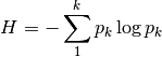
where $p_k$ is the relative abundance of species k

gini-simpson: Calculates the Gini-Simpson coefficient

$D = 1 - \sum_1^k p_k^2$

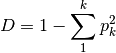
simpon: Calculates Simpson’s D

$D = \sum_1^k p_k^2$

dominance: Dominance index. $\max p_k$

spRich: Species richness (# of non-zero columns)

even: Evenness of a site. Shannon’s H divided by log of species richness.

breakNA: [True | False]

Whether null values should halt the process. If False, then null values are removed from all calculations.

num_equiv: [True | False]

Whether or not species diversity is returned in number-equivalents, which has better properties than raw diversity. Number equivalents are calculated as follows:

shannon: $exp(H)$

gini-simpson: $\frac{1}{1-D}$

simpson: $\frac{1}{D}$

‘spRich’: No conversion needed.

Example

Calculate Shannon diversity of the ‘varespec’ dataset from R:

import ecopy as ep
varespec = ep.load_data('varespec')
shannonH = ep.diversity(varespec, 'shannon')

rarefy(x, method='rarefy', size=None, breakNA=True)¶

Returns either rarefied species richness or draws a rarefaction curve for each row. Rarefied species richness is calculated based on the smallest sample (default) or allows user-specified sample sizes.

Parameters

x: numpy.ndarray or pandas.DataFrame (required)

A site x species matrix, where sites are rows and columns are species.

method: [‘rarefy’ | ‘rarecurve’]

rarefy: Returns rarefied species richness.

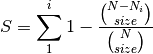
$S = \sum_1^i 1 - \frac{\binom{N-N_i}{size}}{\binom{N}{size}}$

where N is the total number of individuals in the site, $N_i$ is the number of individuals of species i, and size is the sample size for rarefaction

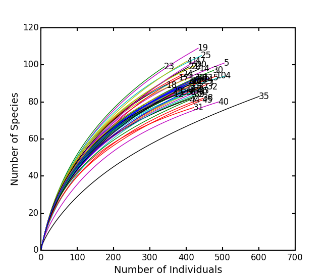
rarecurve: Plots a rarefaction curve for each site (row). The curve is calculated as

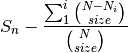
$S_n - \frac{\sum_1^i \binom{N-N_i}{size}}{\binom{N}{size}}$

where $S_n$ is the total number of species in the matrix and size ranges from 0 to the total number of individuals in each site.

Example

Calculate rarefied species richness for the BCI dataset:

import ecopy as ep
BCI = ep.load_data('BCI')
rareRich = ep.rarefy(BCI, 'rarefy')

Show rarefaction curves for each site:

ep.rarefy(BCI, 'rarecurve')

div_partition(x, method='shannon', breakNA=True, weights=None)¶

Partitions diversity into alpha, beta, and gamma components. First, diversity is calculated for each site (see diversity()). Then, a weighted average of each diversity metric is calculated to yield an average alpha diversity. This average alpha diversity is converted to number equivalents $D_\alpha$ (see diversity()). Next, gamma diversity is calculated using the species totals from the entire matrix (i.e. summing down columns) and converted to a number equivalent $D_\gamma$ . Beta diversity is then:

$D_\beta = \frac{D_\gamma} {D_\alpha}$

Parameters

x: numpy.ndarray or pandas.DataFrame (required): A site x species matrix, where sites are rows and columns are species.
method: [‘shannon’ | ‘gini-simpson’ | ‘simpson’ | ‘spRich’]: See diversity()
breakNA: [True | False]: Whether null values should halt the process. If False, then null values are removed from all calculations.
weights: list or np.ndarray: Weights given for each row (site). Defaults to the sum of each row divided by the sum of the matrix. This yields weights based on the number of individuals in a site for raw abundance data or equal weights for relative abundance data.

Example

Partition diversity into alpha, beta, and gamma components for the ‘varespec’ data:

import ecopy as ep
varespec = ep.load_data('varespec')
D_alpha, D_beta, D_gamma = ep.div_partition(varespec, 'shannon')

beta_dispersion(X, groups, test='anova', scores=False, center='median', n_iter=99)¶

Calculate beta dispersion among groups for a given distance matrix. First, the data is subject to transformation as described in PCoA. Next, eigenvalues and eigenvectors are calculated for the transformed matrix. Eigenvectors are split into two matrices, those pertaining to non-negative eigenvalues and those pertaining to negative eigenvalues. Next, centroids for the positive and negative eigenvector matrices are determined (using spatial_median if center=’median’). Z-distances are calculated as:

$z_{ij} = np.sqrt(\delta^2(x_{ij} - c_i^+) - \delta^2(x_{ij}-c_i^-))$

where $\delta^2(x_{ij}, c_i^+)$ is the squared euclidean distance between observation ij and the center of group i, and +/- denote the non-negative and negative eigenvector matrices.

A one-way ANOVA is conducted on the z-distances.

Parameters

X: numpy.ndarray, pandas.DataFrame: A square, symmetric distance matrix
groups: list, pandas.Series, pandas.DataFrame: A column or list containing the group identification for each observation
test: [‘anova’ | ‘permute’]: Whether significance is calculated using the ANOVA approximation or permutation of residuals.
scores: [True | False]: Whether or not the calculated z-distances should be returned for subsequent plotting
center: [‘median’ | ‘centroid’]: Which central tendency should be used for calculating z-distances.
n_iter: integer: Number of iterations for the permutation test

Example

Conduct beta dispersion test on the ‘varespec’ dataset from R:

varespec = ep.load_data('varespec')
dist = ep.distance(varespec, method='bray')

groups = ['grazed']*16 + ['ungrazed']*8
ep.beta_dispersion(dist, groups, test='permute', center='median', scores=False)