Ordination
Ecopy contains numerous methods for ordination, that is, plotting points in reduced space. Techniques include, but are not limited to, principle components analysis (PCA), correspondence analysis (CA), principle coordinates analysis (PCoA), and multidimensional scaling (nMDS).
-
class
pca(x, scale=True, varNames=None)¶ Takes an input matrix and performs principle components analysis. It will accept either pandas.DataFrames or numpy.ndarrays. It returns on object of class :py:class: pca, with several methods and attributes. This function uses SVD and can operate when rows < columns. NOTE: PCA will NOT work with missing observations, as it is up to the user to decide how best to deal with those. Returns object of class
pca.Parameters
- x: a numpy.ndarray or pandas.DataFrame
- A matrix for ordination, where objects are rows and descriptors/variables as columns. Can be either a pandas.DataFrame or numpy. ndarray.
- scale: [True | False]
- Whether or not the columns should be standardized prior to PCA. If ‘True’, the PCA then operates on a correlation matrix, which is appropriate if variables are on different measurement scales. If variables are on the same scale, use ‘False’ to have PCA operate on the covariance matrix.
- varNames: list
- If using a numpy.ndarray, pass a list of column names for to help make PCA output easier to interpret. Column names should be in order of the columns in the matrix. Otherwise, column names are represented as integers during summary.
Attributes
-
evals¶ Eigenvalues in order of largest to smallest.
-
evecs¶ Normalized eigenvectors corresponding to each eigenvalue (i.e. the principle axes).
-
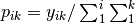
scores¶ Principle component scores of each object (row) on each principle axis. This returns the raw scores
 calculated as
  where
where  is the matrix of eigenvectors and
  are the original observations.
Methods
-
classmethod
summary_imp()¶ Returns a data frame containing information about the principle axes.
-
classmethod
summary_rot()¶ Returns a data frame containing information on axes rotations (i.e. the eigenvectors).
-
classmethod
summary_desc()¶ Returns a data frame containing the cumulative variance explained for each predictor along each principle axis.
-
classmethod
biplot(xax=1, yax=2, type='distance', obsNames=False)¶ Create a biplot using a specified transformation.
- xax: integer
- Specifies which PC axis to plot on the x-axis
- yax: integer
- Specifies which PC axis to plot on the y-axis
- type: [‘distance’ | ‘correlation’]
Type ‘distance’ plots the raw scores
and the raw vectors of the first two principle axes.Type ‘correlation’ plots scores and vectors scaled by the eigenvalues corresponding to each axis:
 and
and  , where
  is a diagonal matrix containing the eigenvalues.
- obsNames: [True | False]
- Denotes whether to plot a scatterplot of points (False) or to actually show the names of the observations, as taken from the DataFrame index (True).
Examples
Principle components analysis of the USArrests data. First, load the data:
import ecopy as ep
USArrests = ep.load_data('USArrests')
USArrests.set_index('State', inplace=True)
Next, run the PCA:
arrests_PCA = ep.pca(USArrests, scale=True)
Check the importance of the different axes by examining the standard deviations, which are the square root of the eigenvalues, and the proportions of variance explained by each axis:
impPC = arrests_PCA.summary_imp()
print(impPC)
            PC1     PC2       PC3     PC4
Std Dev 1.574878 0.994869 0.597129 0.416449
Proportion 0.620060 0.247441 0.089141 0.043358
Cum Prop 0.620060 0.867502 0.956642 1.000000
Next, examine the eigenvectors and loadings to determine which variables contribute to which axes:
rotPC = arrests_PCA.summary_rot()
print(rotPC)
         PC1       PC2     PC3        PC4
Murder 0.535899 0.418181 -0.341233 0.649228
Assault 0.583184 0.187986 -0.268148 -0.743407
UrbanPop 0.278191 -0.872806 -0.378016 0.133878
Rape 0.543432 -0.167319 0.817778 0.089024
Then, look to see how much of the variance among predictors is explained by the first two axes:
print(arrests_PCA.summary_desc())
           PC1      PC2     PC3  PC4
Murder 0.712296 0.885382 0.926900 1
Assault 0.843538 0.878515 0.904153 1
Urban Pop 0.191946 0.945940 0.996892 1
Rape 0.732461 0.760170 0.998626 1
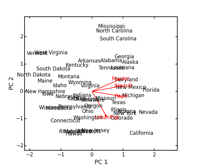
Show the biplot using the ‘correlation’ scaling. Instead of just a scatterplot, use obsNames=True to show the actual names of observations:
arrests_PCA.biplot(type='correlation', obsNames=True)
-
class
ca(x, siteNames=None, spNames=None, scaling=1)¶ Takes an input matrix and performs principle simple correspondence analysis. It will accept either pandas.DataFrames or numpy.ndarrays. Data MUST be 0’s or positive numbers. NOTE: Will NOT work with missing observations, as it is up to the user to decide how best to deal with those. Returns on object of class
ca.Parameters
- x: a numpy.ndarray or pandas.DataFrame
A matrix for ordination, where objects are rows and descriptors/variables as columns. Can be either a pandas.DataFrame or numpy.ndarray. NOTE: If the matrix has more variables (columns) than objects (rows), the matrix will be transposed prior to analysis, which reverses the meanings of the matrices as noted.
The matrix is first scaled to proportions by dividing each element by the matrix sum,
 . Row (site) weights
  are calculated as the sums of row probabilities and column (species) weights
  are the sum of column probabilities. NOTE: If
  in the original matrix, then row weights give species weights and column weights give site weights due to transposition.
A matrix of chi-squared deviations is then calculated as:
This is then converted into a sum-of-squared deviations as

Eigen-decomposition of
 yields a diagonal matrix of eigenvalues and a matrix of eigenvectors . Left-hand eigenvectors
  (as determined by SVD) are calculated as
  . gives the column (species) loadings and gives the row (site) loadings. NOTE: If in the original matrix, the roles of these matrices are reversed.
- siteNames: list
- A list of site names. If left blank, site names are taken as the index of the pandas.DataFrame or the row index from the numpy.ndarray.
- spNames: list
- A list of species names. If left blank, species names are taken as the column names of the pandas.DataFrame or the column index from the numpy.ndarray.
- scaling: [1 | 2]
Which type of scaling to use when calculating site and species scores. 1 produces a site biplot, 2 produces a species biplot. In biplots, only the first two axes are shown. The plots are constructed as follows:
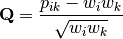
Four matrices are constructed. Outer species (column) locations on CA axes
 are given by the species (column) weights multiplied by the species (column) eigenvalues:
where
 is a diagonal matrix of species (column) weights w_k. Likewise, outer site (row) locations are given by:
Inner site locations
are given as:
Inner species locations are given as:

Scaling 1 Biplot: Scaling 1 shows the relationships among sites within the centroids of the species. This plot is useful for examining relationships among sites and how sites are composed of species. In this, the first two columns of inner site locations
are plotted against the first two columns of the outer species locations . NOTE: If in the original matrix, this will be  and
and  .
.Scaling 2 Biplot: Scaling 2 shows the relationships among species within the centroids of the sites. This plot is useful for examining relationships among species and how species are distributed among sites. In this, the first two columns of inner species locations
are plotted against the first two columns of the outer site locations . NOTE: If in the original matrix, this will be and .
Attributes
-
w_col¶ Column weights in the proportion matrix. Normally species weights unless
 , in which case they are site weights.
-
w_row¶ Row weights in the proportion matrix. Normally site weights unless
, in which case they are species weights.
-
U¶ Column (species) eigenvectors (see above note on transposition).
-
Uhat¶ Row (site) eigenvectors (see above note on transposition).
-
cumDesc_Sp¶ pandas.DataFrame of the cumulative contribution of each eigenvector to each species. Matrix
is scaled by eigenvalues  . Then, the cumulative sum of each column is divided by the column total for every row. If in the original data, then this operation is performed on automatically.
-
cumDesc_Site¶ The same for cumDesc_Sp, but for each site. Normally calculated for
unless , then calculated on .
-
siteScores¶ Site scores along each CA axis. All considerations for matrix transposition and scaling have been taken into account.
-
spScores¶ Species scores along each CA axis. All considerations for matrix transposition and scaling have been taken into account.
Methods
-
classmethod
summary()¶ Returns a pandas.DataFrame of summary information for each correspondence axis, including SD’s (square-root of each eigenvalue), proportion of inertia explained, and cumulative inertia explained.
-
classmethod
biplot(coords=False, type=1, xax=1, yax=2, showSp=True, showSite=True, spCol='r', siteCol='k', spSize=12, siteSize=12, xlim=None, ylim=None)¶ Produces a biplot of the given CA axes.
- xax: integer
- Specifies CA axis to plot on the x-axis.
- yax: integer
- Specifies CA axis to plot on the y-axis.
- showSp: [True | False]
- Whether or not to show species in the plot.
- showSite: [True | False]
- Whether or not to show sites in the plot.
- spCol: string
- Color of species text.
- siteCol: string
- Color of site text.
- spSize: integer
- Size of species text.
- siteSize: integer
- Size of site text.
- xlim: list
- A list of x-axis limits to override default.
- ylim: list
- A list of y-axis limits to override default.
Examples
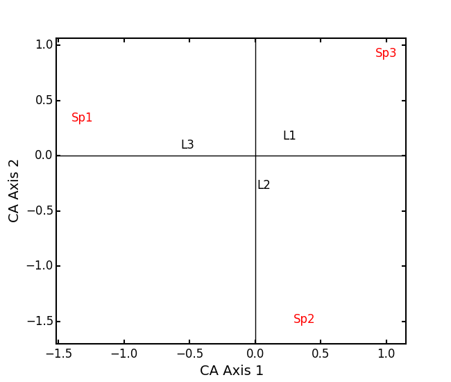
In Legendre and Legendre (2012), there is an example of three species varying among three lakes. Write in that data:
import ecopy as ep
import numpy as np
import pandas as pd
Lakes = np.array([[10, 10, 20], [10, 15, 10], [15, 5, 5]])
Lakes = pd.DataFrame(Lakes, index = ['L1', 'L2', 'L3'])
Lakes.columns = ['Sp1', 'Sp2', 'Sp3']
Next, run the CA:
lakes_CA = ep.ca(Lakes)
Check the variance explained by each CA axis (there will only be two):
CA_summary = lakes_CA.summary()
print(CA_summary)
          CA Axis 1 CA Axis 2
Std. Dev 0.310053 0.202341
Prop. 0.701318 0.298682
Cum. Prop. 0.701318 1.000000
Next, see how well the two axes explained variance in species and sites:
print(lakes_CA.cumDesc_Sp)
   CA Axis 1 CA Axis 2
Sp1 0.971877 1
Sp2 0.129043 1
Sp3 0.732340 1

print(lakes_CA.cumDesc_site)
    CA Axis 1 CA Axis 2
L1 0.684705 1
L2 0.059355 1
L3 0.967209 1
Make a Type 1 biplot to look at the relationship among sites:
lakes_CA.biplot()
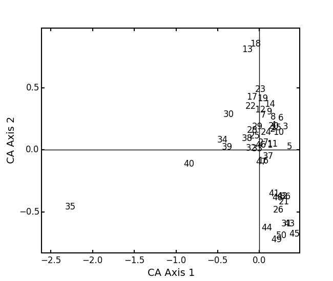
In a bigger example, run CA on the BCI dataset. NOTE: This is an example where
:BCI = ep.load_data('BCI') bci_ca = ep.ca(BCI) bci_ca.biplot(showSp=False)
-
class
pcoa(x, correction=None, siteNames=None)¶ Takes a square-symmetric distance matrix with no negative values as input. NOTE: This will not work with missing observations. Returns an object of class
pcoa.Parameters
- x: a numpy.ndarray or pandas.DataFrame
A square, symmetric distance matrix with no negative values and no missing observations. Diagonal entries should be 0.
For PCoA, distance matrix
 is first corrected to a new matrix
  , where
  . Elements of the new matrix are centered by row and column means using the equation
  . PCoA is eigenanalysis of
  . Eigenvectors are scaled by the square root of each eigenvalue
  where is a diagonal matrix of the eigenvalues.
- correction: [None | 1 | 2]
Which correction should be applied for negative eigenvalues. Accepts either ‘1’ or ‘2’ (must be a string). By default, no correction is applied.
Correction 1: Computes PCoA as described above. Adds the absolute value of the largest negative eigenvalue to the square original distance matrix (while keeping diagonals as 0) and then re-runs PCoA from the beginning.
Correction 2: Constructs a special matrix

 is the centered, corrected distance matrix as described above and
  is a centered matrix (uncorrected) of
  . The largest, positive eigenvalue of this matrix is then added the original distances and PCoA run from the beginning.
- siteNames: list
- A list of site names. If not passed, inherits from the DataFrame index or assigns integer values.
Attributes
-
evals¶ Eigenvalues of each principle coordinate axis.
-
U¶ Eignevectors describing each axis. These have already been scaled.
-
correction¶ The correction factor applied to correct for negative eignvalues.
Methods
-
classmethod
summary()¶ Returns a pandas.DataFrame summarizing the variance explained by each principle coordinate axis.
-
classmethod
biplot(coords=False, xax=1, yax=2, descriptors=None, descripNames=None, spCol='r', siteCol='k', spSize=12, siteSize=12)¶ Produces a biplot of the given PCoA axes.
- coords: [True | False]
- If True, returns a dictionary of the plotted axes, where ‘Objects’ gives the coordinates of objects and ‘Descriptors’ gives the coordinates of the descriptors, if any.
- xax: integer
- Specifies PCoA axis to plot on the x-axis.
- yax: integer
- Specifies PCoA axis to plot on the y-axis.
- descriptors: numpy.ndarray or pandas.DataFrame
An n x m matrix of descriptors to plot on the biplot. These can be the original descriptors used to calculate distances among objects or an entirely new set. Descriptors must be quantitative. It will work for binary descriptors, but may be meaningless.
Given a new matrix
of descriptors, the matrix is standardized by columns to produce a new matrix  . The given principle coordinate axes denoted by xax and yax are placed into an n x 2 matrix , which is also standardized by column. The covariance between the new descriptors and principle coordinates is given by
The covariance
 is then scaled by the eigenvalues corresponding to the given eigenvectors:
Matrix
 contains the coordinates of each descriptor and is what is returned as ‘Descriptors’ if coords=True.
- descripNames: list
- A list containing the names of each descriptor. If None, inherits from the column names of the pandas.DataFrame or assigned integer values.
- spCol: string
- Color of species text.
- siteCol: string
- Color of site text.
- spSize: integer
- Size of species text.
- siteSize: integer
- Size of site text.
-
classmethod
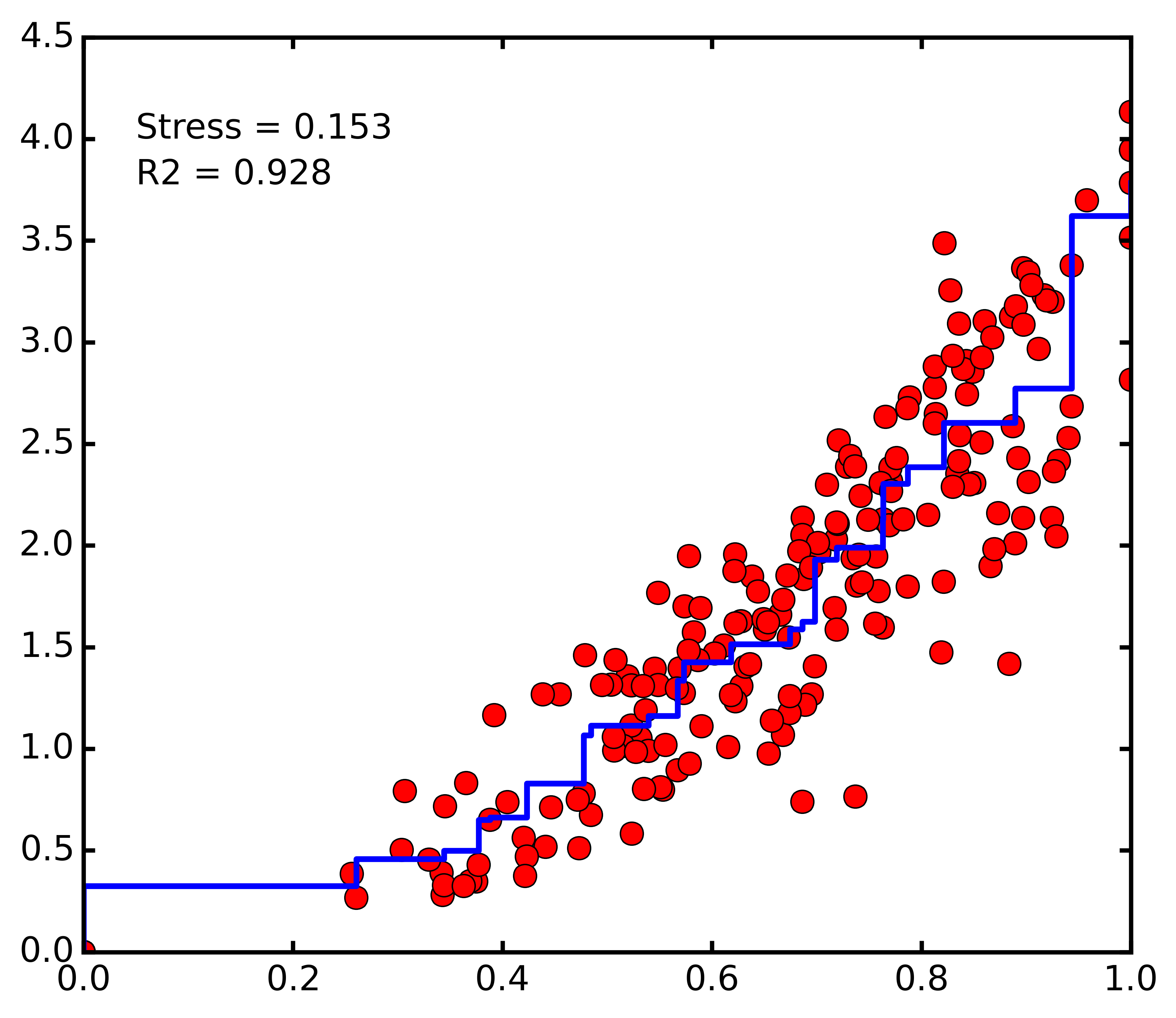
shepard(xax=1, yax=2)¶ Plots a Shepard diagram of Euclidean distances among objects in reduced space vs. original distance calculations. xax and yax as above.
Examples
Run PCoA on the ‘BCI’ data:
import ecopy as ep

BCI = ep.load_data('BCI')
brayD = ep.distance(BCI, method='bray', transform='sqrt')
pc1 = ep.pcoa(brayD)
print(pc1.summary()[['PCoA Axis 1', 'PCoA Axis 2']])

        PCoA Axis 1 PCoA Axis 2
Std. Dev 1.094943 0.962549
Prop. 0.107487 0.083065
Cum. Prop. 0.107487 0.190552

pc1.biplot()
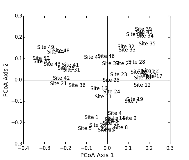
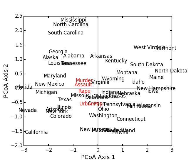
Attempting to show species on the above biplot results in a messy graph. To better illustrate its use, run PCoA on the USArrests data:
USA = ep.load_data('USArrests')
USA.set_index('State', inplace=True)
# standardize columns first
USA = USA.apply(lambda x: (x - x.mean())/x.std(), axis=0)
eucD = ep.distance(USA, 'euclidean')

pc2 = ep.pcoa(eucD, siteNames=USA.index.values)
pc2.biplot(descriptors=USA)
-
class
MDS(distmat, siteNames=None, naxes=2, transform='monotone', ntry=20, tolerance=1E-4, maxiter=3000, init=None)¶ Takes a square-symmetric distance matrix with no negative values as input. After finding the solution that provide the lowest stress, ecopy.MDS scales the fitted distances to have a maximum equal to the maximum observed distance. Afterwards, it uses PCA to rotate the object (site) scores so that variance is maximized along the x-axis. Returns an object of class
MDS.Parameters
- distmat: np.ndarray or pandas.DataFrame
- A square-symmetric distance matrix.
- siteNames: list
- A list of names for each object. If none, takes on integer values or the index of the pandas.DataFrame.
- naxes: integer
- Number of ordination axes.
- transform: [‘absolute’ | ‘ratio’ | ‘linear’ | ‘monotone’]
Which transformation should be used during scaling.
absolute: Conducts absolute MDS. Distances between points in ordination space should be as close as possible to observed distances.
ratio: Ordination distances are proportional to observed distances.
linear: Ordination distances are a linear function of observed distances. Uses the technique of Heiser (1991) to avoid negative ordination distances.
monotone: Constrains ordination distances simply to be ranked the same as observed distance. Typically referred to as non-metric multidimensional scaling. Uses isotonic regression developed by Nelle Varoquaux and Andrew Tulloch from scikit-learn.
- ntry: integer
- Number of random starts used to avoid local minima. The returned solution is the one with the lowest final stress.
- tolerance: float
- Minimum step size causing a break in the minimization of stress. Default = 1E-4.
- maxiter: integer
- Maximum number of iterations to attempt before breaking if no solution is found.
- init: numpy.ndarray
- Initial positions for the first random start. If none, the initial position of the first try is taken as the site locations from classical scaling, Principle Coordinates Analysis.
Attributes
-
scores¶ Final scores for each object along the ordination axes.
-
stress¶ Final stress.
-
obs¶ The observed distance matrix.
-
transform¶ Which transformation was used.
Methods
-
classmethod
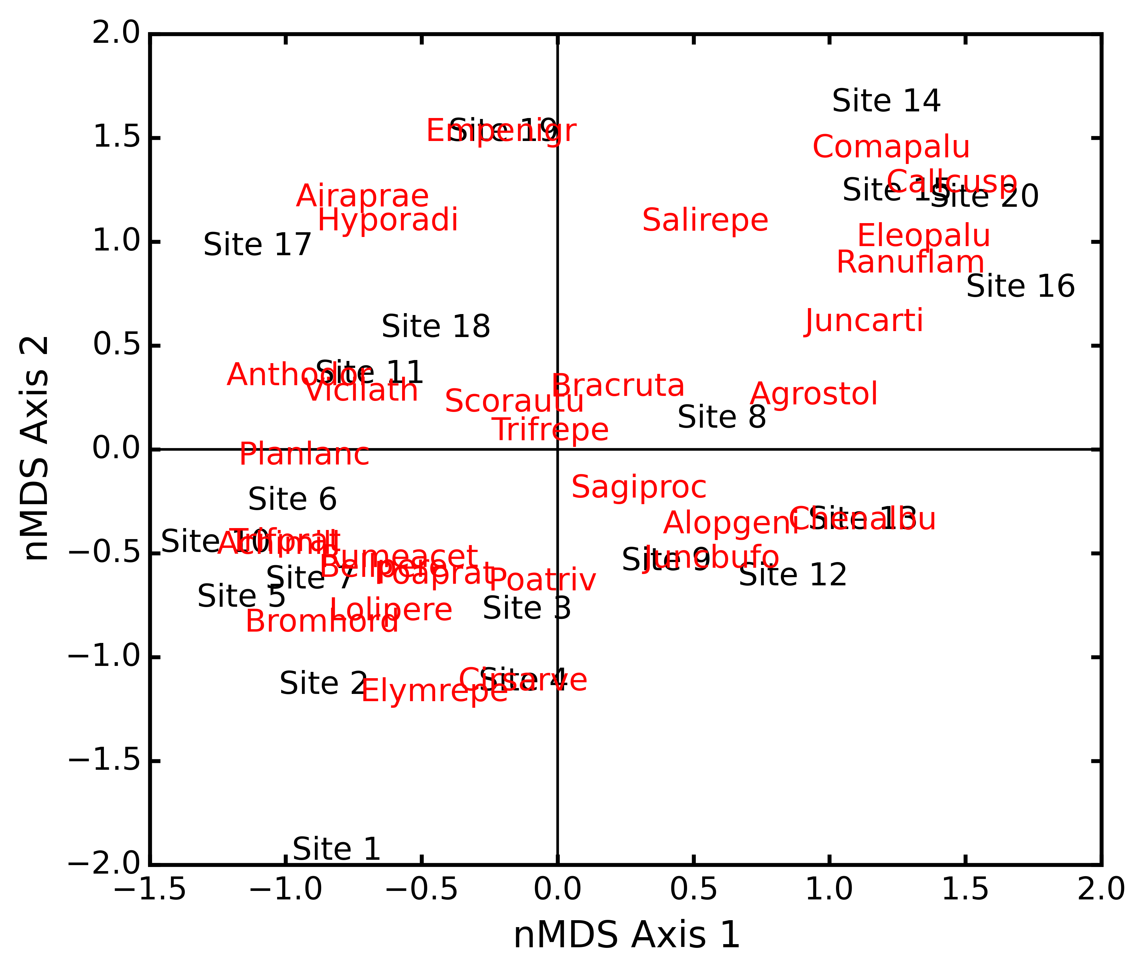
biplot(coords=False, xax=1, yax=2, siteNames=True, descriptors=None, descripNames=None, spCol='r', siteCol='k', spSize=12, siteSize=12)¶ Produces a biplot of the given MDS axes.
- coords: [True | False]
- If True, returns a dictionary of the plotted axes, where ‘Objects’ gives the coordinates of objects and ‘Descriptors’ gives the coordinates of the descriptors, if any.
- xax: integer
- Specifies MDS axis to plot on the x-axis.
- yax: integer
- Specifies MDS axis to plot on the y-axis.
- descriptors: numpy.ndarray or pandas.DataFrame
- A matrix of the original descriptors used to create the distance matrix. Descriptors (i.e. species) scores are calculated as the weighted average of site scores.
- descripNames: list
- A list containing the names of each descriptor. If None, inherits from the column names of the pandas.DataFrame or assigned integer values.
- spCol: string
- Color of species text.
- siteCol: string
- Color of site text.
- spSize: integer
- Size of species text.
- siteSize: integer
- Size of site text.
-
classmethod
shepard(xax=1, yax=2)¶ Plots a Shepard diagram of Euclidean distances among objects in reduced space vs. original distance calculations. xax and yax as above.
-
classmethod
correlations()¶ Returns a pandas.Series of correlations between observed and fitted distances for each site.
-
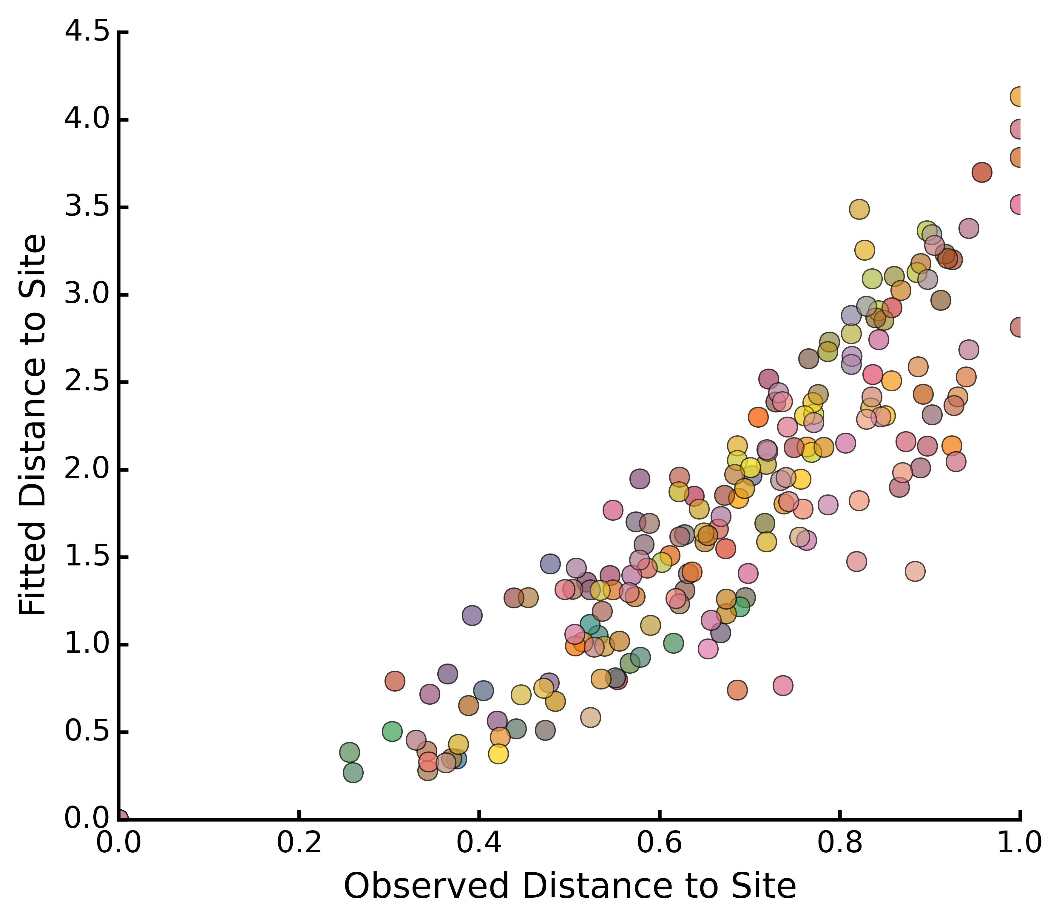
classmethod
correlationPlots(site=None)¶ Produces a plot of observed vs. fitted distances for a given site. If site=None, then all sites are plotted on a single graph.
Examples
Conduct nMDS on the ‘dune’ data:
import ecopy as ep
dunes = ep.load_data('dune')
dunes_T = ep.transform(dunes, 'wisconsin')
dunes_D = ep.distance(dunes_T, 'bray')
dunesMDS = ep.MDS(dunes_D, transform='monotone')
Plot the Shepard diagram:
dunesMDS.shepard()
Check the correlations for observed vs. fitted distances:
dunesMDS.correlationPlots()
Make a biplot, showing species locations:
dunesMDS.biplot(descriptors=dunes_T)
-
class
hillsmith(mat, wt_r=None, ndim=2)¶ Takes an input matrix and performs ordination described by Hill and Smith (1976). Returns an object of class
hillsmith, with several methods and attributes. NOTE: This will NOT work when rows < columns or with missing values.Parameters
- mat: pandas.DataFrame
- A matrix for ordination, where objects are rows and descriptors/variables as columns. Can have mixed data types (both quantitative and qualitative). If all columns are quantitative, this method is equivalent to PCA. If all columns are qualitative, this method is equivalent to MCA. Should not be used with ordered factors. In order to account for factors, this method creates dummy variables for each factor and then assigns weights to each dummy column based on the number of observations in each column.
- wt_r: list or numpy.ndarray
- Optional vector of row weights.
- ndim: int
- Number of axes and components to save.
Attributes
-
evals¶ Eigenvalues in order of largest to smallest.
-
pr_axes¶ The principle axes of each column.
-
row_coords¶ Row coordinates along each principle axis.
-
pr_components¶ The principle components of each row.
-
column_coords¶ Column coordinates along each principle component.
Methods
-
classmethod
summary()¶ Returns a data frame containing information about the principle axes.
-
classmethod
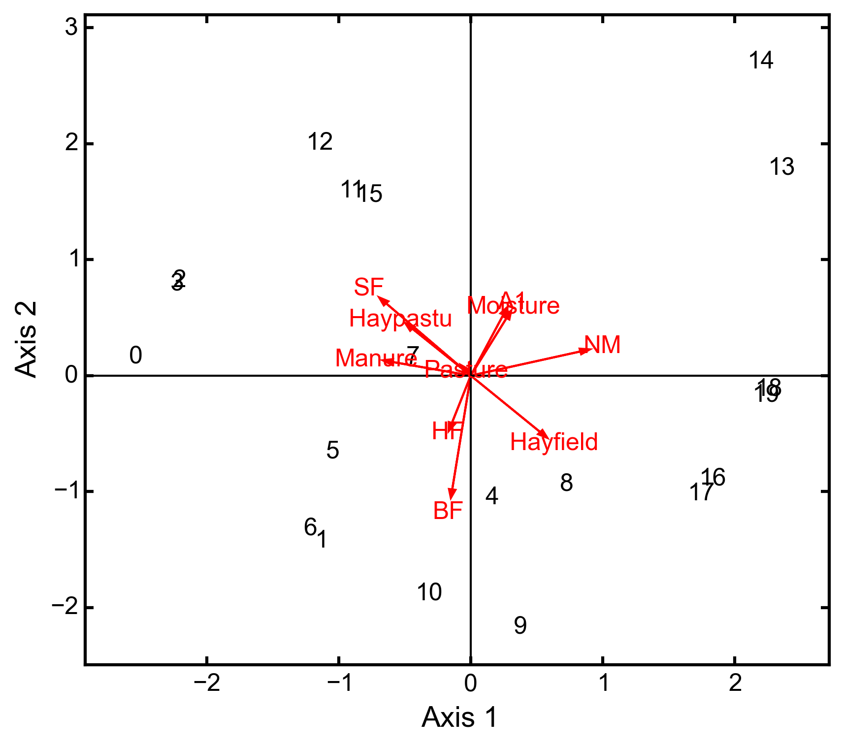
biplot(invert=False, xax=1, yax=2, obsNames=True)¶ Create a biplot using a specified transformation.
- invert: [True|Fasle]
- If False (default), plots the row coordinates as points and the principle axes of each column as arrows. If True, plots the column coordinates as points and the principle components of each row as arrows.
- xax: integer
- Specifies which PC axis to plot on the x-axis.
- yax: integer
- Specifies which PC axis to plot on the y-axis.
- obsNames: [True | False]
- Denotes whether to plot a scatterplot of points (False) or to actually show the names of the observations, as taken from the DataFrame index (True).
Examples
Hill and Smith analysis of the dune_env data:
import ecopy as ep
dune_env = ep.load_data('dune_env')
dune_env = dune_env[['A1', 'Moisture', 'Manure', 'Use', 'Management']]
print(ep.hillsmith(dune_env).summary().iloc[:,:2])

                        Axis 1    Axis 2
        Std. Dev  1.594392  1.363009
        Prop Var  0.317761  0.232224
        Cum Var   0.317761  0.549985

ep.hillsmith(dune_env).biplot(obsNames=False, invert=False)
-
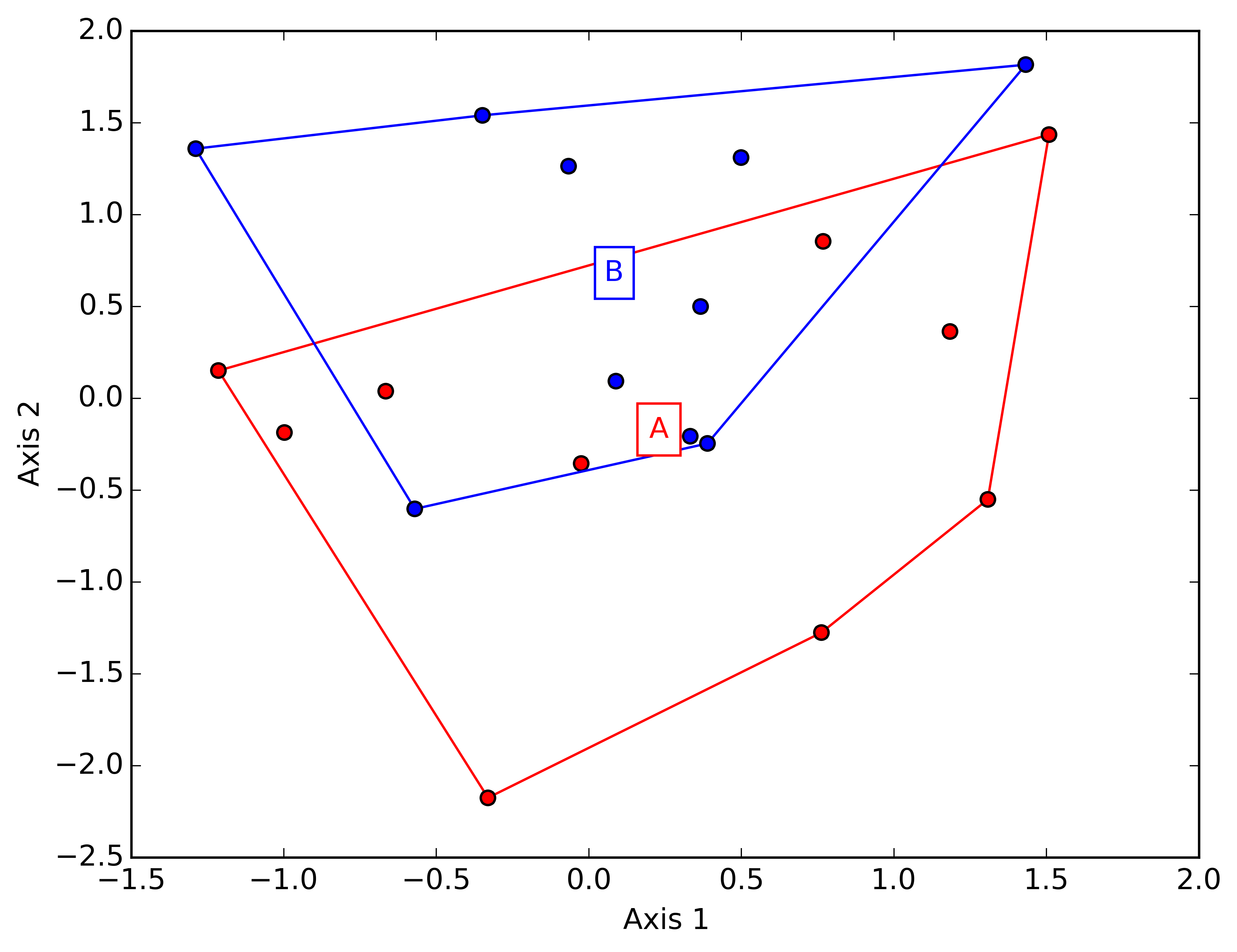
ord_plot(x, groups, y=None, colors=None, type='Hull', label=True, showPoints=True, xlab='Axis 1', ylab='Axis 2')¶ Delineates different groups in ordination (or regular) space.
Parameters
- x: numpy.ndarray, pandas.DataFrame, pandas.Series (required)
- Coordinates to be plotted. Can be either a one or two column matrix. If only one column, then y must be specified.
- groups: list, pandas.DataFrame, pandas.Series (required)
- Factor denoting group identification
- y: numpy.ndarray, pandas.DataFrame, pandas.Series
- y coordinates to be plotted. Can only have one column, and must be specified is x is only one column.
- colors: string, list, pandas.Series, pandas.DataFrame
- Gives custom colors for each group. Otherwise default colors are used.
- type: [‘Hull’ | ‘Line’]
- ‘Hull’ produces a convex hull, whereas ‘Line’ produces lines connected to the centroid for each point.
- label: [True | False]
- Whether or not a label should be shown at the center of each group.
- showPoints: [True | False]
- Whether or not the points should be shown.
- xlab: string
- Label for the x-axis.
- ylab: string
- Label for the y-axis.
Example
Generate fake data simulating ordination results:
import numpy as np
import ecopy as ep
import matplotlib.pyplot as plt

nObs = 10
X = np.random.normal(0, 1, 10*2)
Y = np.random.normal(0, 1, 10*2)
GroupID = ['A']*nObs + ['B']*nObs

Z = np.vstack((X, Y)).T
Make a convex hull plot where groups are red and blue:
ep.ord_plot(x=Z, groups=GroupID, colors=['r', 'b'])
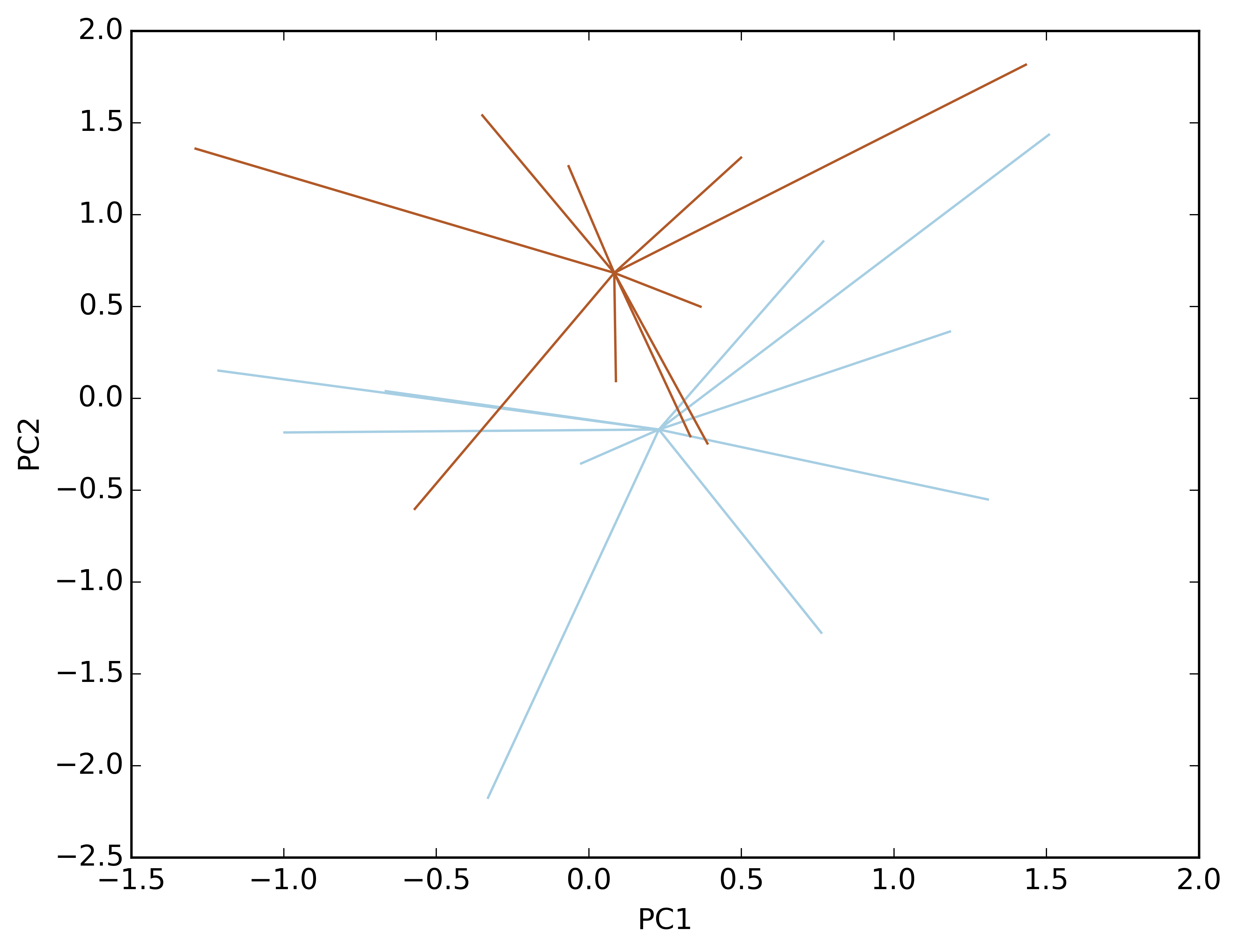
Make a line plot with coordinates in different matrices. Remove the points and the labels:
ep.ord_plot(x=X, y=Y, groups=GroupID, type='Line', xlab='PC1', ylab='PC2', showPoints=False, label=False)